这篇博客是论文:High Accuracy Optical Flow Estimation Based Theory for Warp 的笔记,论文为2004年,在2015年EpicFlow方法中引用。
在稠密光流估计中,最后一步往往是将光流图进行Refine和smooth,来确保光流在空间上连续,大部分区域符合刚体运动假设,同时也会处理遮挡,为遮挡区域提供连续的光流值。
在介绍的论文中,建立了一个能量函数,将光流图的优化和优化能量函数联系起来。论文偏向传统,但是也很经典,接下来一起看下做法。
一、灰度恒常假设
我们假设参与光流计算的两张图,保持了大致恒定的亮度(即亮度相同),如果记 I 为图像矩阵,t和t+1时刻的运动向量用w=(u,v,1)表示,假设平移不改变亮度:
I(x,y,t)=I(x+u,y+u,t+1)
进一步引出光流算法中经常会用到的约束:(下标表示偏导)
I_xu+I_yu+I_t=0
二、梯度恒常假设
灰度恒常性假设有一个很大的缺陷,当光照变化时假设就不再成立,而图像中的运动常常伴随着光照变化。于是我们对上式做出一些改变,不再假设灰度恒定,而假设位移前后的梯度恒定,那么可以给出:
\nabla I(x,y,t)=\nabla I(x+u,y+v,t+1) \\ where \nabla=(\partial_x,\partial_y)^T
该假设较灰度恒常假设更具有一般性。
三、平滑假设
在估计局部光流时,很少考虑周围或者更远的像素,只在局部进行光流估计通常会忽略领域或者全局像素之间的关联。对于刚性的运动,通常相临近的位置光流值的变化是连续的。如果局部光流估计不准确,可能会出现outlier点。
于是平滑假设这样描述,我们假定在物体内部,通常是练成一片的区域内,光流值在空间上连续变化。而在物体边界,光流值会产生突变。
四、多尺度策略
我们通常会使用coast-to-fine的策略,或者多尺度策略来处理光流问题。大运动或者噪声情况下,光流在downsample的小图上处理通常更加有效。
五、灰度恒常和梯度恒常的能量函数
我们定义 gamma 作为权重,灰度恒常性和梯度恒常性的代价函数可以写成如下形式:
E_{Data}(u,v)=\int_\Omega(|I(x+w)-I(x)|^2+\gamma|\nabla I(x+w)-\nabla I(x)|^2)dx我们考虑到outliner点会带来巨大影响,于是我们增加一个带有正则项的函数psi(s^2),来增加代价函数的鲁棒性
E_{Data}(u,v)=\int_\Omega\Psi(|I(x+w)-I(x)|^2+\gamma|\nabla I(x+w)-\nabla I(x)|^2)dx \\ \Psi(s^2)=\sqrt{s^2+\epsilon^2}六、平滑性约束的能量函数
平滑性约束,就是对物体内部光流(u,v)的一致性做约束,写成能量函数可以做如下表达
E_{Smooth}(u,v)=\int_\Omega\Psi(|\nabla_3u|^3+|\nabla_3v|^3)dx \\ \nabla_3=(\partial_x,\partial_y,\partial_t)^T七、总的能量函数
我们的目标是找到u,v,使如下能量函数的值最小(其中alpha>0,调节两项的相对权重)
E(u,v)=E_{Data}+\alpha E_{Smooth}八、欧拉-拉格朗日方程
根据费马引理,一个连续函数取极值的必要条件是它的导函数等于0。我们将函数这一定义推广到泛函,可以得到泛函的极值条件,也就是欧拉-拉格朗日方程。
前面能量函数 E(u,v) 是高度非线形的,所以方程没有平凡解。
我们用z替换t,考虑时域上是不可导的,所有没有z的偏导数,我们规定如下记号
I_x=\partial_xI(x+w) \\
I_y=\partial_yI(x+w) \\
I_z=I(x+w)-I(x) \\
I_{xx}=\partial_{xx}I(x+w) \\
I_{xy}=\partial_{xy}I(x+w) \\
I_{yy}=\partial_{yy}I(x+w) \\
I_{xz}=\partial_xI(x+w)-\partial_xI(x) \\
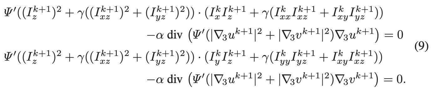
I_{yz}=\partial_yI(x+w)-\partial_yI(x) 能量方程的优化必须完全满足欧拉-拉格朗日方程,于是它x和y的导函数满足:
x:\\ \\
\Psi'(I_z^2+\gamma(I_{xz}^2+I_{yz}^2)) \circ(I_xI_z+\gamma(I_{xx}I_{xz}+I_{xy}I_{yz}))\\-\alpha \ {div} (\Psi'(|\nabla_3u|^2+|\nabla_3v|^2)\nabla_3u)=0
\\ \\
y:
\\ \\
\Psi'(I_z^2+\gamma(I_{xz}^2+I_{yz}^2)) \circ(I_yI_z+\gamma(I_{yy}I_{yz}+I_{xy}I_{xz}))\\-\alpha \ {div} (\Psi'(|\nabla_3u|^2+|\nabla_3v|^2)\nabla_3u)=0
九、解的数值近似
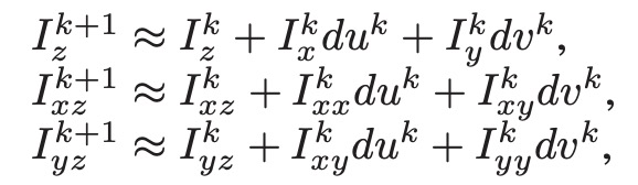
实际求解过程可以采用金字塔coast-to-fine的方式求解,先求解整数部分,再求解小数部分。我们用k表示帧序号,那么上式z用k表达可写作下式。
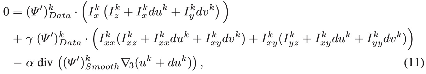
因为z的偏导数是非线形的,为了移除非线形,我们对与z相关的偏导数进行泰勒一阶展开,我们只取一阶项,解uv的问题就被转换成了线形方程组的求解。
代入上述公式,合并smooth项和data项
我们用 l 表示我们内层迭代中每一步的初值(步数标号),那么式子可以写成。
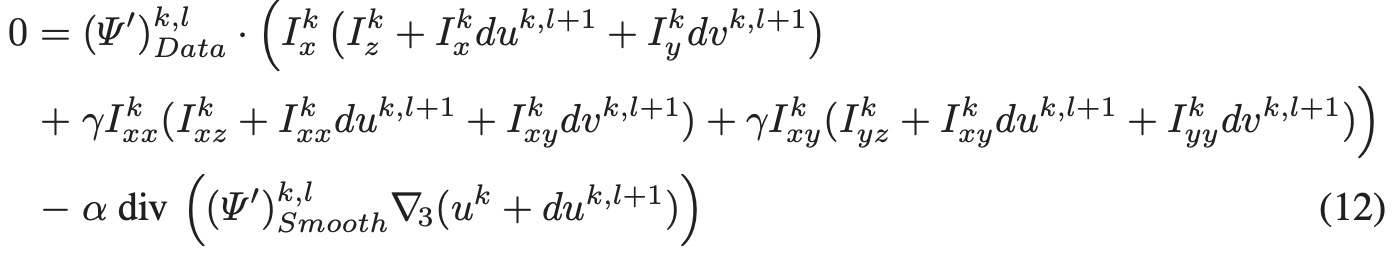
上面的方程因为已经丢掉z偏导的高阶项,所以是一个线形方程组,可以用 Gauss-Seidel 法或者 SOR (successive over relaxation)迭代求解。
Gauss-Seidel迭代可以参考:线性方程组-迭代法 2:Jacobi迭代和Gauss-Seidel迭代 – 知乎 (zhihu.com)
SOR可以参考:逐次超松弛SOR迭代概述 – 知乎 (zhihu.com)
十、代码
代码可以从epic.cpp的论文连接中获取,这里以epic 代码中的variationc.pp进行解释
首先是variation.cpp的入口,首先是设置参数,然后对参与计算的两张图进行平滑,然后送入compute_one_level进行处理计算。
/* Compute a refinement of the optical flow (wx and wy are modified) between im1 and im2 */
void variational(image_t *wx, image_t *wy, const color_image_t *im1, const color_image_t *im2, variational_params_t *params){

    // Check parameters
    if(!params){
        params = (variational_params_t*) malloc(sizeof(variational_params_t));
        if(!params){
          fprintf(stderr,"error: not enough memory\n");
          exit(1);
        }
        variational_params_default(params);
    }

    // initialize global variables
    half_alpha = 0.5f*params->alpha;
    half_gamma_over3 = params->gamma*0.5f/3.0f;
    half_delta_over3 = params->delta*0.5f/3.0f;

    float deriv_filter[3] = {0.0f, -8.0f/12.0f, 1.0f/12.0f};
    deriv = convolution_new(2, deriv_filter, 0);
    float deriv_filter_flow[2] = {0.0f, -0.5f};
    deriv_flow = convolution_new(1, deriv_filter_flow, 0);


    // presmooth images
    int width = im1->width, height = im1->height, filter_size;
    color_image_t *smooth_im1 = color_image_new(width, height), *smooth_im2 = color_image_new(width, height);
    float *presmooth_filter = gaussian_filter(params->sigma, &filter_size);
    convolution_t *presmoothing = convolution_new(filter_size, presmooth_filter, 1);
    color_image_convolve_hv(smooth_im1, im1, presmoothing, presmoothing);
    color_image_convolve_hv(smooth_im2, im2, presmoothing, presmoothing);
    convolution_delete(presmoothing);
    free(presmooth_filter);

    compute_one_level(wx, wy, smooth_im1, smooth_im2, params);

    // free memory
    color_image_delete(smooth_im1);
    color_image_delete(smooth_im2);
    convolution_delete(deriv);
    convolution_delete(deriv_flow);
}
接下来在 compute one level 函数中,首先compute_dpsis_weight 在梯度图上计算局部smooth权重,然后开始迭代求解光流。
迭代分为内层迭代和外层迭代,内层迭代中,首先按照本次迭代的初始光流值对图像进行warp,本次迭代在此基础上求解残差。然后求解计算x,y,z(t)方向的偏导数。
内层迭代中,就开始计算能量函数的 data item 和 smooth item,然后sor_couple函数求解得到光流值。
/* perform flow computation at one level of the pyramid */
void compute_one_level(image_t *wx, image_t *wy, color_image_t *im1, color_image_t *im2, const variational_params_t *params){
    const int width = wx->width, height = wx->height, stride=wx->stride;

    image_t *du = image_new(width,height), *dv = image_new(width,height), // the flow increment
        *mask = image_new(width,height), // mask containing 0 if a point goes outside image boundary, 1 otherwise
        *smooth_horiz = image_new(width,height), *smooth_vert = image_new(width,height), // horiz: (i,j) contains the diffusivity coeff from (i,j) to (i+1,j)
        *uu = image_new(width,height), *vv = image_new(width,height), // flow plus flow increment
        *a11 = image_new(width,height), *a12 = image_new(width,height), *a22 = image_new(width,height), // system matrix A of Ax=b for each pixel
        *b1 = image_new(width,height), *b2 = image_new(width,height); // system matrix b of Ax=b for each pixel

    color_image_t *w_im2 = color_image_new(width,height), // warped second image
        *Ix = color_image_new(width,height), *Iy = color_image_new(width,height), *Iz = color_image_new(width,height), // first order derivatives
        *Ixx = color_image_new(width,height), *Ixy = color_image_new(width,height), *Iyy = color_image_new(width,height), *Ixz = color_image_new(width,height), *Iyz = color_image_new(width,height); // second order derivatives


    image_t *dpsis_weight = compute_dpsis_weight(im1, 5.0f, deriv);

    int i_outer_iteration;
    for(i_outer_iteration = 0 ; i_outer_iteration < params->niter_outer ; i_outer_iteration++){
        int i_inner_iteration;
        // warp second image
        image_warp(w_im2, mask, im2, wx, wy);
        // compute derivatives
        get_derivatives(im1, w_im2, deriv, Ix, Iy, Iz, Ixx, Ixy, Iyy, Ixz, Iyz);
        // erase du and dv
        image_erase(du);
        image_erase(dv);
        // initialize uu and vv
        memcpy(uu->data,wx->data,wx->stride*wx->height*sizeof(float));
        memcpy(vv->data,wy->data,wy->stride*wy->height*sizeof(float));
        // inner fixed point iterations
        for(i_inner_iteration = 0 ; i_inner_iteration < params->niter_inner ; i_inner_iteration++){
            //  compute robust function and system
            compute_smoothness(smooth_horiz, smooth_vert, uu, vv, dpsis_weight, deriv_flow, half_alpha );
            compute_data_and_match(a11, a12, a22, b1, b2, mask, du, dv, Ix, Iy, Iz, Ixx, Ixy, Iyy, Ixz, Iyz, half_delta_over3, half_gamma_over3);
            sub_laplacian(b1, wx, smooth_horiz, smooth_vert);
            sub_laplacian(b2, wy, smooth_horiz, smooth_vert);
            // solve system
            sor_coupled(du, dv, a11, a12, a22, b1, b2, smooth_horiz, smooth_vert, params->niter_solver, params->sor_omega);
            // update flow plus flow increment
            int i;
            v4sf *uup = (v4sf*) uu->data, *vvp = (v4sf*) vv->data, *wxp = (v4sf*) wx->data, *wyp = (v4sf*) wy->data, *dup = (v4sf*) du->data, *dvp = (v4sf*) dv->data;
            for( i=0 ; i<height*stride/4 ; i++){
                (*uup) = (*wxp) + (*dup);
                (*vvp) = (*wyp) + (*dvp);
                uup+=1; vvp+=1; wxp+=1; wyp+=1;dup+=1;dvp+=1;
	        }
        }
        // add flow increment to current flow
        memcpy(wx->data,uu->data,uu->stride*uu->height*sizeof(float));
        memcpy(wy->data,vv->data,vv->stride*vv->height*sizeof(float));
    }
    // free memory
    image_delete(du); image_delete(dv);
    image_delete(mask);
    image_delete(smooth_horiz); image_delete(smooth_vert);
    image_delete(uu); image_delete(vv);
    image_delete(a11); image_delete(a12); image_delete(a22);
    image_delete(b1); image_delete(b2);
    image_delete(dpsis_weight);
    color_image_delete(w_im2);
    color_image_delete(Ix); color_image_delete(Iy); color_image_delete(Iz);
    color_image_delete(Ixx); color_image_delete(Ixy); color_image_delete(Iyy); color_image_delete(Ixz); color_image_delete(Iyz);
}
sor求解,如果是单次迭代,会调用到下面的代码:
void sor_coupled_slow_but_readable(image_t *du, image_t *dv, const image_t *a11, const image_t *a12, const image_t *a22, const image_t *b1, const image_t *b2, const image_t *dpsis_horiz, const image_t *dpsis_vert, const int iterations, const float omega){
    int i,j,iter;
    float sigma_u,sigma_v,sum_dpsis,A11,A22,A12,B1,B2,det;
    for(iter = 0 ; iter<iterations ; iter++){
        for(j=0 ; j<du->height ; j++){
	        for(i=0 ; i<du->width ; i++){
	            sigma_u = 0.0f;
	            sigma_v = 0.0f;
	            sum_dpsis = 0.0f;
	            if(j>0){
		            sigma_u -= dpsis_vert->data[(j-1)*du->stride+i]*du->data[(j-1)*du->stride+i];
		            sigma_v -= dpsis_vert->data[(j-1)*du->stride+i]*dv->data[(j-1)*du->stride+i];
		            sum_dpsis += dpsis_vert->data[(j-1)*du->stride+i];
		        }
	            if(i>0){
                    sigma_u -= dpsis_horiz->data[j*du->stride+i-1]*du->data[j*du->stride+i-1];
                    sigma_v -= dpsis_horiz->data[j*du->stride+i-1]*dv->data[j*du->stride+i-1];
                    sum_dpsis += dpsis_horiz->data[j*du->stride+i-1];
		        }
	            if(j<du->height-1){
		            sigma_u -= dpsis_vert->data[j*du->stride+i]*du->data[(j+1)*du->stride+i];
		            sigma_v -= dpsis_vert->data[j*du->stride+i]*dv->data[(j+1)*du->stride+i];
		            sum_dpsis += dpsis_vert->data[j*du->stride+i];
		        }
	            if(i<du->width-1){
		            sigma_u -= dpsis_horiz->data[j*du->stride+i]*du->data[j*du->stride+i+1];
		            sigma_v -= dpsis_horiz->data[j*du->stride+i]*dv->data[j*du->stride+i+1];
		            sum_dpsis += dpsis_horiz->data[j*du->stride+i];
		        }
                A11 = a11->data[j*du->stride+i]+sum_dpsis;
                A12 = a12->data[j*du->stride+i];
                A22 = a22->data[j*du->stride+i]+sum_dpsis;
                det = A11*A22-A12*A12;
                B1 = b1->data[j*du->stride+i]-sigma_u;
                B2 = b2->data[j*du->stride+i]-sigma_v;
                du->data[j*du->stride+i] = (1.0f-omega)*du->data[j*du->stride+i] +omega*( A22*B1-A12*B2)/det;
                dv->data[j*du->stride+i] = (1.0f-omega)*dv->data[j*du->stride+i] +omega*(-A12*B1+A11*B2)/det;
	        }
	    }
    }
}
更细致的过程可以参考原始论文或者epicflow代码。